Methods for Conceptual Capital Cost Estimation

By Clayton T. Baumann, PE, CCP, ASA | evcValuation and Christopher T. Rigo | evcValuation

Click HERE to download a PDF version of this article

Abstract

Conceptual capital-cost estimates are important for assessing the economic viability of proposed projects, but their usefulness depends on understanding how to appropriately apply the estimates.

Introduction

Capital cost estimates are a crucial step in order to make prudent decisions regarding any development project. Specifically, the economic viability of a development project must be sufficiently supported in order to move forward in the planning process. In the early phases of a development project cost engineers are often engaged in developing conceptual capital cost estimates for various types of industrial facilities like chemical plants, production units, or even individual pieces of equipment. A major hurdle cost engineers can encounter is identifying facilities or production units that are similar to apply as benchmarks or pricing reference points. Even when other existing facilities or production units are similar in many aspects, it is very common that the facility or production unit being considered for development differs materially in technology, capacity, location, or the time of construction. In such instances, an understanding of how to appropriately apply conceptual capital cost estimating methods is critical.

This article briefly discusses various conceptual capital cost estimating methods. It then presents a detailed discussion and example on one method for conceptual capital cost estimating, the cost-to-capacity method also commonly referred to as the capacity factored estimating technique. Further, the appropriate application of scale factors (also commonly referred to as scaling exponents, scaleup exponents, cost-capacity factors, cost to capacity factors, and capacity factors) utilized in the cost-to-capacity method is presented, along with applicable methodology for scale factor derivations.

Conceptual Capital Cost Estimating Methods

As identified by the Association for the Advancement of Cost Engineering (“AACE”) International, there are five classes of costs estimates, Class 1 through Class 5. A Class 1 cost estimate is the most detailed and is based on a fully defined project scope, while a Class 4 or Class 5 estimate is more conceptual in nature and is based on more limited information and a project scope that is not fully defined [1, 2, 3].

There are multiple commonly utilized conceptual capital cost estimating methods which would be considered a Class 4 or Class 5 estimate including, but not limited to [4]:

• Cost-to-Capacity Estimating Method (also referred to capacity factored method) – Historical or current capital cost data for a similar project but with a different capacity is utilized with a non-linear scaling exponent as the primary basis for the cost estimate of the proposed project.
• End-Product Units Estimating Method – Historical capital cost data for similar projects are utilized in conjunction with units of capacity to apply a linear relationship as the primary basis for the estimate of a proposed project.
• Physical Dimensions Estimating Method – Historical capital cost data for similar projects are utilized in conjunction with physical dimensions to apply a linear relationship as the primary basis for the estimate of a proposed project.
• Analogy Estimating Method – Historical capital cost data for similar projects with similar capacities are utilized as the primary basis for the estimate of a proposed project.
• Expert Judgement Estimating Method – Primarily utilized when there is no reasonably similar project for comparison or available capital costs, the judgement of subject matter experts is utilized as the primary basis for the estimate of the proposed project.

Cost-to-Capacity Methodology Overview

Among the previously presented conceptual capital cost estimating methods, the cost-to-capacity method is one of the most utilized and easy to apply. Yet, the method is often not fully understood, and commonly applied in an inappropriate and inconsistent manner in conceptual cost estimating analyses.
The cost-to-capacity concept was originally applied in 1947 by Roger Williams Jr. to develop equipment cost estimates; later, in 1950, C.H. Chilton expanded the concept’s application to estimate total chemical plant costs [3, 5].

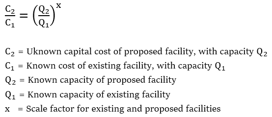
The fundamental concept behind the cost-to-capacity method is that the costs of similar facilities, production units, or pieces of equipment with different capacities vary nonlinearly. More specifically, cost is a function of capacity raised to an exponent or scale factor [3,6]. The governing equation is as follows:

The scale factor in the above equation accounts for the nonlinear relationship and introduces the concept of economies of scale where, as a facility becomes larger, the incremental cost is reduced for each additional unit of capacity [3, 7]. However, not all facilities, production units, or pieces of equipment actually experience economies of scale related to capital costs. A scale factor of less than 1 indicates that economies of scale exist and the incremental cost of the next added unit of capacity will be cheaper than the previous unit of capacity. When the scale factor is greater than 1, economies of scale do not exist; rather, diseconomies of scale exist, and the incremental cost becomes more expensive for every added unit of capacity. A scale factor of exactly 1 indicates that a linear relationship exists and there is no change in the incremental cost per unit of added capacity [3, 8]. A scale factor of 1 also indicates that it is just as economically feasible to build two small facilities as one large facility with the same capacity [3, 4].

Cost-to-Capacity Methodology Considerations

One of the main advantages of the cost-to-capacity method is its relatively easy application. It can be applied to quickly develop reasonable order-of-magnitude capital cost estimates. Potentially even more useful is its capacity to allow sensitivity analyses to be quickly performed when high degrees of accuracy are not required [3, 4]. However, there are a number of considerations that must be addressed prior to applying the cost-to-capacity method [3].

To obtain reasonable results, the technology of the development facility should be the same as, or very close to, that of the existing facility with a known capital cost. Likewise, the scale factor that is applied must appropriately reflect both the technology of the existing facility and the development facility. As will subsequently be discussed in more detail, the scale factor that is applied should also be specifically applicable to the range of capacities for the specific technology of existing facility and development facility [3].

In addition to technology, the cost engineer must consider the configuration of the existing and development facility, their location, and any unique design and site characteristics of each. Differences in location would almost always require the application of a locational cost adjustment factor. (There are many various sources that publish location-based indices that can be used for making location adjustments including: Compass International Estimating Yearbooks, Marshall and Swift (“M&S”), RSMeans Cost Manuals, Engineering News-Record, and U.S. Department of Defense publications, to name a few. To develop a location adjustment factor, the same basic equation that is subsequently presented for making time adjustments is applicable.) Likewise, different configurations or unique design or site characteristics of the existing or development facility would require a cost adjustment prior to completing the cost-to-capacity analysis. Significant differences between the existing and development facility in any of the aforementioned areas can yield nonmeaningful capital cost estimates [3, 7].

Lastly, prior to applying the cost-to-capacity method, the known capital costs of the existing facility that have a specified reference year must be appropriately adjusted for inflation in order to develop a reliable cost estimate for the proposed facility. For example, it may be required to develop a capital cost estimate for a proposed chemical facility in current dollars but the known capital costs of the similar existing reference facility are in 2020 dollars. In general terms, to appropriately account for the effects of cost inflation, the known capital costs for the existing facility must be escalated using appropriate cost indices applicable to the technology in question [3, 7]. In this example, the known capital costs for the existing facility must be multiplied by a ratio of the current year index and the 2020 index [3, 6].

The following equation illustrates the general relationship:

When using cost indices to escalate known capital costs there are some nuances to be aware of. The older the known capital costs are, the greater potential there is to have diminished accuracy in the capital cost estimate of the proposed facility. Thus, known capital costs for existing facilities that are escalated for inflation using the previously presented equation need to be analyzed to determine whether they are still appropriate and relevant. When estimating capital costs for a development facility, the use of known capital costs for existing facilities that are as current as possible will typically yield more meaningful results [3, 6].

Some commonly used, reliable cost indices that can be applied in escalating known capital costs for existing facilities include the following: Handy-Whitman Index of Public Utility Construction Costs, Engineering News-Record (“ENR”) Construction Cost Index, Nelson-Farrar Refinery Cost Index, IHS Downstream Capital Cost Index (“DCCI”), Chemical Engineering’s Plant Cost Index, and Marshall and Swift (“M&S”) Cost Index [3].

Cost-to-Capacity Method Example

A simple application example of the cost-to-capacity method is given below in order to better illustrate the previously discussed concepts and methodologies:

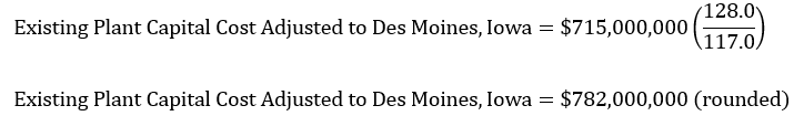
A conceptual capital cost estimate is needed for the proposed development of 1,500 tons/day ammonia plant near Des Moines, Iowa as of a current date. There are known capital cost for a similar plant of the same technology located near Houston, Texas with a capacity of approximately 1,000 tons/day which had construction completed in January 2022. The total capital cost of the existing plant in January 2022 dollars was approximately $715,000,000. It is concluded that the existing plant is very similar to the proposed plant and employs the same process technology so no cost adjustment is required for unique design characteristics. However, due to the fact that proposed facility is located in a different region than the existing facility a location adjustment is required. Additionally, an adjustment must be made to the known capital costs in January 2022 dollars for time/inflation in order to get a cost estimate as of a current date. Lastly, an adjustment must be made for the difference in capacities of the existing and proposed facilities by utilizing the cost-to-capacity method.

First, the known capital costs for the existing ammonia plant located near Houston, Texas must be adjusted to get to an estimate of the capital costs if had been constructed near Des Moines, Iowa. A location index applicable to the chemical industry indicates a location index of 117.0 for Houston, Texas and a location index of 128.0 for Des Moines, Iowa. Applying the two indices in a formula similar to the time adjustment formula is shown below:

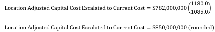
Next, the location adjusted capital costs which are still in January 2022 dollars must be converted to current dollars. An applicable cost index for the chemical industry indicates a January 2022 index value of 1085.0 and a current date index value of 1180.0. Applying the two indices in the previously presented formula is presented below:

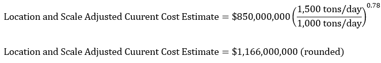
Lastly, the location adjusted time escalated cost must be scaled to account for the difference in capacities between the proposed and existing ammonia. A credible source indicates that an appropriate scale factor to apply in cost estimates for an ammonia plant is 0.78. The previously introduced equation for the cost-to-capacity method can now be mathematically manipulated and solved as follows:

As shown in the above cost estimate example, a capacity increase of 1.5 times results in a capital cost increase of approximately 1.37 times. This expresses the previously introduced concept of economies of scale inherent in applying a scale factor of less than 1 [3].

Scale Factor Derivation Methodology

One of most crucial components when applying the cost-to-capacity method is an appropriate scale factor. The previously mentioned study performed by C.H. Chilton in 1950 derived a common scale factor for chemical facilities of approximately 0.6, which led to the cost-to-capacity method being referred to early on as the “six-tenths rule” [3, 8]. Since the Chilton study, many other sources have published scale factors for various industrial facilities and equipment of certain technologies. However, the majority of these scale factors are not published with supporting industry data and derivations [3].

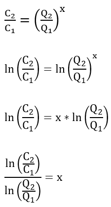
The methodology for deriving a scale factor is similar in nature to the cost-to-capacity method equation as previously presented. If cost and capacity data are known for different facilities, production units, or prices of equipment with the same or very similar technology and design, then a scale factor can be derived. The previously presented equation for the cost-to-capacity method can easily be transformed by applying natural logarithms (“ln”) to the cost and capacity data on both sides of the equation to develop a linear relationship. It can then be further manipulated to solve for the non-linear scale factor, x. The below equations show this relationship [3].

The above relationship outlines the basic concept behind the development of a linear relationship and the derivation of a scale factor. However, in order to derive a more accurate scale factor for a particular facility, production unit, or piece of equipment with a certain technology, an entire set of capital cost and capacity data must be available and analyzed. To accomplish this, natural logarithms can be applied to an entire set of cost and capacity data and then graphed. A linear regression analysis of the natural logarithm of the cost and capacity data can then be performed using graphing computer software. The resultant linear regression line slope is the representative scale factor for that particular type of facility with a specific technology [3, 8].

It is important that the cost and capacity data that is gathered and analyzed in the linear regression analysis is consistent with respect to design parameters such as technology, configuration, location, and unique site characteristics. These are similar to the considerations of the cost-to-capacity method, as previously stated [3].

Scale Factor Derivation Example

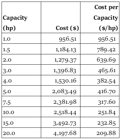
An example is best to illustrate and understand the derivation of a scale factor using regression analysis. The table below presents the capacity and associated cost and cost per horsepower for different capacities of horizontal centrifugal pumps in current dollars. The data set is for the off the shelf cost for horizontal centrifugal pumps from the same manufacturer and is concluded to be an acceptable data set because it has consistent cost information. (When deriving a scale factor for an entire facility or production unit, the most reliable data set is one that is consistent and has the same or very similar basic manufacturer designs, location basis, technology, and configuration. If there are variations in the costs that make up the data set in relation to any of these attributes, certain adjustments may need to be made prior to performing the scale factor derivation.) It should be noted that the methodology presented in the following example is universal and can apply to any data set for known capital costs and capacities for entire facilities, production units, or pieces of equipment.

Table 1 – Horizontal Centrifugal Pump Capacities and Costs [9]

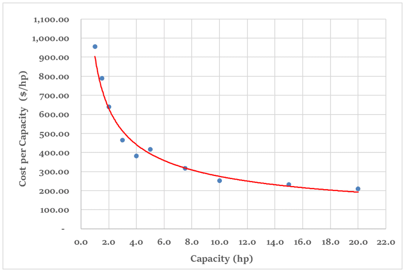
The data above in Table 1 illustrates a declining trend in the cost per horsepower (“hp”) of capacity as the size of the horizontal centrifugal pump increases which demonstrates the concept of economies of scale that exist as capacity increases. Figure 1 below provides a visual depiction of the declining cost per horsepower of capacity.

Figure 1 – Horizontal Centrifugal Pump Cost per Capacity vs. Capacity [9]

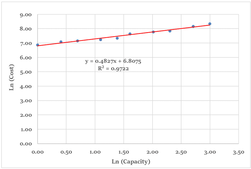
The relationship of economies of scale that exists for horizontal centrifugal pumps is what is captured when deriving the scale factor for the above data set. As previously described, in order to derive a scale factor from the above data set, natural logarithms are applied to both the cost and capacity data and then graphed. A linear regression analysis is then performed on the natural logarithm of the total cost and capacity to derive a linear regression equation. Figure 2 below shows a graph of the natural logarithm of the cost and capacity data from Table 1, along with the resultant linear regression equation [3].

Figure 2 – Horizontal Centrifugal Pump Natural Logarithm of Cost vs. Natural Logarithm Capacity

Per the linear regression equation shown in Figure 2 above, the slope of the line is 0.4827. As previously discussed, this slope is representative of the scale factor for the given set of cost and capacity data analyzed. Thus, the derived scale factor for horizontal centrifugal pump for the range of capacities analyzed is concluded to be approximately 0.48, rounded.

R² values calculated in linear regression analyses are indicators of how closely a linear regression line approximates a given set of data. The closer the R² value is to 1, the better the regression line estimates the data set. By visual inspection, the linear regression equation appears to closely match the set of data. Furthermore, the R² shown in Figure 2 above is 0.9722, indicating that the linear regression equation is a good approximate for the data set [3].

Scale Factor Considerations

The previously presented scale factor derivation for the cost and capacity data for the horizontal centrifugal pump is a simplified example in that one scale factor was derived for a range of horsepower capacities. Depending on the type of technology of the particular facility, production unit, or piece of equipment, the scale factor could increase at certain ranges of capacity due to fixed increases in costs for larger capacities [3, 10]. In many cases, if a set of cost and capacity data is broken down into subsets and a scale factor derivation is performed, the resultant scale factors for the larger capacity subsets could be greater than the smaller capacity subsets. Thus, caution should be used when deriving a single scale factor based on broad ranges of capacities for a particular facility, production unit, or piece of equipment. Understanding that scale factors may vary over ranges of capacities should cause a level of caution to be taken when applying a single scale factor in cost-to-capacity analyses for a broad range of facility, production unit, or equipment capacity. Utilizing a scale factor that is not appropriate for a given range of capacities will lead to less reliable conceptual capital cost estimate results [3].

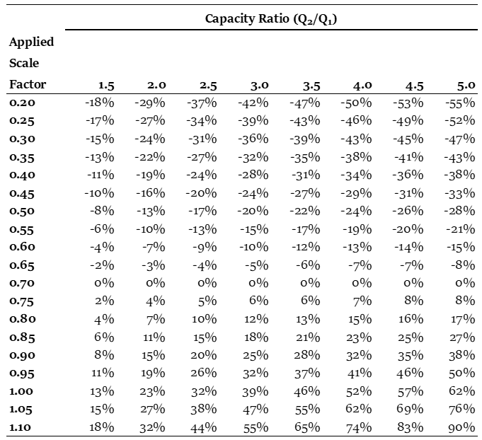
For illustrative purposes, assume a conceptual capital cost estimate is undertaken for a development project and the appropriate scale factor to apply for the given facility of a certain technology and capacity is 0.70. The table below presents the potential percent error inherent in the capital cost estimate if the scale factor applied in the analysis deviates from 0.70.

Table 2 – Capacity Ratio (Q₂/Q₁)

The above table shows that the use of an inappropriate scale factor can introduce significant error. Thus, it is critical that the scale factor applied in the cost-to-capacity method should be supported by publications or derivations and should apply to the technology and range of capacities applicable to the capital cost estimate in order to yield a reliable capital cost estimation [11].

Conclusion

Conceptual capital cost estimates can be useful tools when making decisions early on in the planning process for a development project when only a limited project scope exists. In order to arrive at reasonable capital cost estimates, cost engineers must be aware of the various conceptual cost estimating methods that exists and certain consideration associated with each. The cost-to-capacity method is one tool that can allow cost engineers to develop conceptual capital cost estimates for entire facilities, production units, or pieces of equipment based on known capital costs for similar assets with different capacities. While mathematically, the cost-to-capacity method is fairly simplistic, it must be applied in a consistent and appropriate manner in order to produce meaningful results. Analyzing and utilizing cost data for facilities, production units, or equipment that are not adequately similar to the subject of the cost estimate, or applying a scale factor that is arbitrary or not appropriate, can result in a significant under- or overstatement of the capital cost estimate. However, when applied appropriately, the cost-to-capacity method can yield fairly quick and reliable conceptual capital cost estimates which can be critical in determining the economic feasibility of a development project.

References

1. AACE International Recommended Practice No. 17R-97, “Cost Estimate Classification System,” AACE International, Morgantown, WV, August 7, 2020, pp. 2-3.
2. AACE International Recommended Practice No. 10S-90, “Cost Engineering Terminology,” AACE International, Morgantown, WV, July 24, 2024, pp. 36-37.
3. Baumann, Clayton T., “Cost-to-Capacity Method: Applications and Considerations,” The Journal of the International Machinery & Technical Specialties Committee of the American Society of Appraisers, Volume 30, Issue 1 (1^st Quarter 2014), pp. 49 – 56.
4. Dysert, Larry R., and Elliott, Bruce G., “Early Conceptual Estimating Methodologies,” Cost Engineering, vol. 63, no. 01, AACE International, Morgantown, WV, January/February 2021, pp. 30 – 39.
5. Remer, Donald S., “Design Cost Factors for Scaling-up Engineering Equipment,” Chemical Engineering Progress, August 1990, p. 77.
6. Humphreys, Kenneth K., Jelen’s Cost and Optimization Engineering, McGraw-Hill, Inc., New York, NY, 1991, pp. 382-387.
7. S. Department of Energy, National Energy Technology Laboratory, Systems Engineering & Analysis Directorate, “Quality Guidelines for Energy Systems Studies, Capital Cost Scaling Methodology: Revision 3 Reports and Prior,” April 1, 2019, pp. 12 – 16. Retrieved from https://www.netl.doe.gov/energy-analysis/details?id=3741.
8. Ellsworth, Richard K., “Cost to Capacity Factor Development for Facility Projects,” Cost Engineering, vol. 49, no. 9, Sept. 2007, p. 27.
9. “Centrifugal Pump Price List,” 2024 inverter.com, Retrieved from https://www.inverter.com/centrifugal-pump-price-list.
10. Chase, David J., “Plant Cost vs. Capacity: New Way to Use Exponents”, Modern Cost Engineering: Methods and Data, McGraw-Hill Publishing Co., New York, NY, 1979, pp. 228-229.
11. Baumann, Clayton T. and Lopatnikov, Alexander, “Scaling Laws: Uses and Misuses in Industrial Plant and Equipment Replacement Cost Estimates,” The Journal of the International Machinery & Technical Specialties Committee of the American Society of Appraisers, Volume 33, Issue 2 (2^nd Quarter 2017), pp. 38 – 44.

This article was previously published in Chemical Engineering magazine.